WTE2 (part 1) - 3D tracking of particles inside an evaporating droplet

In this tutorial you will learn to apply DefocusTracker to measure flows in a real application. You will find the 3D position of tracer particles at different time instant and then apply a tracking method to obtain velocity and particle trajectories. Finally you will scale the data to obtain results in physical units. You can read more detail on the experimental setup in Rossi et al., Phys. Rev. E 100, 033103 (2019).

0 - Instruction
1 - Create and train the model
2 - Validate the model on the training data
3 - Check the processing parameters on a subset of data
4 - Check the tracking parameters on a subset of data
5 - Scale the data to real units
6 - Run the full processing on all datasets
7 - Save the data
Bibliography

0 - Instruction

Install DefocusTracker (see the README.md file)
Complete WTE0 and WTE1.
Download the Datasets-WTE2 and unzip it into the folder 'workthrough-examples//Datasets-WTE2/'.
Follow the instructions and run this script cell-by-cell using the command (Ctrl+Enter).

1 - Create and train the model

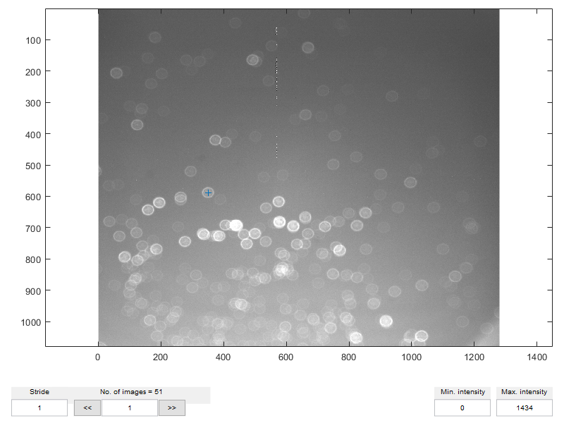
Experimental training images are typically taken by scanning along z tracer particles at fixed location (e.g. particle sedimented on the bottom of a microchannel)

In comparison with WTE1 we used here more advanced features with smoothing and interpolation. We smoothed the calibration images and interpolate them to obtain 100 images from 51. You can try to vary these parameters (smoothing typically between 0.1 and 0.2, n_inter_images typically no more than 100) to improve the results in noisy data.

clc, clear, close all

%  Load the training images:
myfolder = './/Datasets-WTE2/Scan-step2um//';
img_train = dtracker_create('imageset',myfolder);

%  Create the training dataset
N_cal = img_train.n_frames;
dat_train = dtracker_create('dataset',N_cal);
dat_train.fr(:) = 1:N_cal;
dat_train.X(:) = zeros(1,N_cal) + 350; %350 is the X-coord. of the selected particle
dat_train.Y(:) = zeros(1,N_cal) + 588; %855 is the Y-coord. of the selected particle
dat_train.Z(:) = linspace(0,1,N_cal);

%  Inspect the training set
dtracker_show(img_train,dat_train)

Create the model with default parameters

model_wte2 = dtracker_create('model');

%  Edit the relevant field in training parameters
model_wte2.training.imwidth = 45;            % width of the particle image
model_wte2.training.imheight = 39;           % height of the particle image
model_wte2.training.median_filter = 3;       % median filter to reduce thermal noise
model_wte2.training.smoothing = 0.2;         % smoothing (optional)
model_wte2.training.n_interp_images = 100;   % interpolation (optional)

%  Train the *model*
model_wte2 = dtracker_train(model_wte2,img_train,dat_train);

%  Inspect the *model*
dtracker_show(model_wte2)

Training started ...
Training done! Total Time: 1.9 secs

2 - Validate the model on the training data

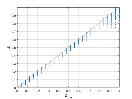
You can obtain a first validation of your model by running a processing on the full training data. Since the particles in one frame are all lying in the same physical plane, you can determine the true Z position of the particles as a function the frame number.

model_wte2.processing.cm_guess = .5;
model_wte2.processing.cm_final = .9;
dat_valid = dtracker_process(model_wte2,img_train,1:2:N_cal);

Evaluation started ...
1/26 - 7 s - 4 particles - time left: 3 mins, 3.5 secs
2/26 - 7 s - 37 particles - time left: 2 mins, 50.4 secs
3/26 - 6 s - 53 particles - time left: 2 mins, 22.7 secs
4/26 - 7 s - 67 particles - time left: 2 mins, 42.7 secs
5/26 - 7 s - 89 particles - time left: 2 mins, 28.8 secs
6/26 - 7 s - 106 particles - time left: 2 mins, 22.0 secs
7/26 - 8 s - 118 particles - time left: 2 mins, 28.7 secs
8/26 - 7 s - 124 particles - time left: 2 mins, 5.9 secs
9/26 - 7 s - 127 particles - time left: 2 mins, 4.4 secs
10/26 - 8 s - 133 particles - time left: 2 mins, 13.5 secs
11/26 - 7 s - 140 particles - time left: 1 min, 43.4 secs
12/26 - 7 s - 143 particles - time left: 1 min, 44.0 secs
13/26 - 8 s - 147 particles - time left: 1 min, 41.0 secs
14/26 - 7 s - 152 particles - time left: 1 min, 20.2 secs
15/26 - 7 s - 155 particles - time left: 1 min, 20.4 secs
16/26 - 7 s - 156 particles - time left: 1 min, 6.7 secs
17/26 - 7 s - 159 particles - time left: 1 min, 4.6 secs
18/26 - 7 s - 154 particles - time left: 57.5 secs
19/26 - 6 s - 153 particles - time left: 44.2 secs
20/26 - 7 s - 148 particles - time left: 41.4 secs
21/26 - 7 s - 146 particles - time left: 34.0 secs
22/26 - 7 s - 140 particles - time left: 27.3 secs
23/26 - 7 s - 144 particles - time left: 21.4 secs
24/26 - 7 s - 147 particles - time left: 13.9 secs
25/26 - 7 s - 137 particles - time left: 7.2 secs
26/26 - 7 s - 75 particles - time left:  
----------------------------
Evaluation done! Total Time: 3 mins, 4.8 secs

figure
plot((dat_valid.fr-1)/(N_cal-1),dat_valid.Z,'.',[0 1],[0 1])
grid on
xlabel('Z_{true}')
ylabel('Z')

3 - Check the processing parameters on a subset of data

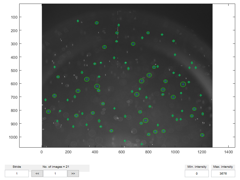
You can now run the processing on the experimental images. In this tutorial experimental images are tracer particles inside an evaporating droplets. The setup and physics of the experiment is described in Rossi et al., Phys. Rev. E 100, 033103 (2019).

Before running the experiment on the full dataset, it is a good idea to try it on few images and adjust the parameters.

%  Load the experimental images
myfolder = './/Datasets-WTE2/Drop-UPW//';
img_exp = dtracker_create('imageset',myfolder);

%  Set the processing parameters and run the evluation on the first 4 frames
model_wte2.processing.cm_guess = .5;
model_wte2.processing.cm_final = .9;
dat_exp = dtracker_process(model_wte2, img_exp, 1:3);

%  Inspect the results and change setting if not satisfied.
dtracker_show(dat_exp, img_exp)

Evaluation started ...
1/3 - 7 s - 83 particles - time left: 14.7 secs
2/3 - 7 s - 79 particles - time left: 7.2 secs
3/3 - 8 s - 85 particles - time left:  
----------------------------
Evaluation done! Total Time: 22.1 secs

4 - Check the tracking parameters on a subset of data

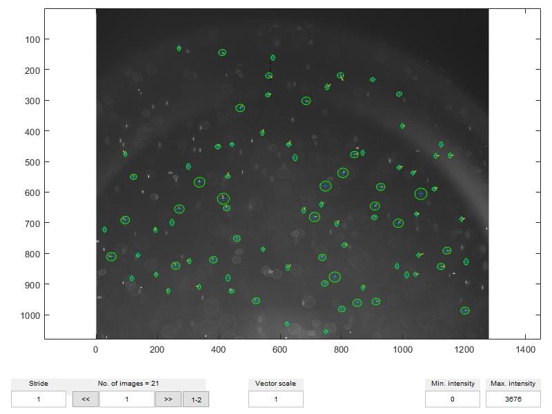
After we have determined the 3D position of the particles, we want to track their displacement to calculate their velocity and trajectory. In DefocusTracker, you can use the function dtracker_postprocess() to apply a tracking scheme to a dataset. As for the processing, you need to create a tracking data stucture first, change the suitable parameters, and then apply it to a dataset. The default tracking scheme in DefocusTracker is the nearest neighbor approach. This has only 2 parameters:

tracking_step, that indicates after how many frames we are searching the particles to connect. In this case (tracking_step = 1), we connect particles in one frame with particles to the next frame.
bounding_box, that indicate the minimum and maximum allowed displacement in X, Y, and Z direction, respectivealy.

tracking_wte2 = dtracker_create('tracking');
tracking_wte2.tracking_step = 1;
tracking_wte2.bounding_box = [-30 30 -30 30 -0.12 0.12]; %  [DXmin DXmax DYmin DYmax DZmin DZmax]
dat_exp_track = dtracker_postprocess(tracking_wte2,dat_exp);

dtracker_show(dat_exp_track, img_exp)

Tracking - nearest neighbor - started...
Tracking done! Total time: 0 min 0 sec

5 - Scale the data to real units

After image processing, the particle positions X,Y,Z and corresponding displacements DX,DY,DZ are given in normalized units. X and Y are normalized with the size of an image pixel, whereas Z is normalized with the measurement depth. To obtain the value of position and velocity in real units, we need to calculate the scaling factors:

x = X*(camera pixel size)/(magnification in X-direction)
y = Y*(camera pixel size)/(magnification in Y-direction)
z = Z*(number of frames in the training set - 1)*step length*refractive index of the fluid
vx = DX*(camera pixel size)/(magnification in X-direction)/Dt
vy = DY*(camera pixel size)/(magnification in X-direction)/Dt
vz = DZ*(number of frames in the training set - 1)*step length* refractive index of the fluid/Dt

Dt is the time between two frames. In DefocusTracker you can create a scaling structure and then apply to the dataset using the function dtracker_postprocess().

%  Create a default scaling and edit the relevant fields
scaling_wte2 = dtracker_create('scaling');
scaling_wte2.X_to_x = 1.2659;
scaling_wte2.Y_to_y = 1.1965;
scaling_wte2.Z_to_z = -(N_cal-1)*2*1.33;
scaling_wte2.dt = 10;
scaling_wte2.unit = 'um';

%  Apply the scaling
dat_exp_track_scaled = dtracker_postprocess('scale',dat_exp_track,scaling_wte2);

Note the different variable names in a dataset are different if it is scaled (uppercase) or unscaled (lowercase).

disp(head(dat_exp_track,5))

    fr      X         Y          Z          DX         DY          DZ       id      cm   
    __    ______    ______    _______    ________    _______    ________    __    _______

    1      443.2     444.1    0.72139           0          0           0     0    0.99337
    1     248.04    698.84    0.95361           0          0           0     0    0.98714
    1     442.39    922.93    0.62879     -6.9661    -8.3465    0.040108    45    0.97347
    1       1013    869.68    0.93768           0          0           0     0    0.98204
    1     121.99    549.72    0.49054    0.040107    -5.0668    0.071196    11    0.98497

disp(head(dat_exp_track_scaled,5))

    fr      x         y         z          vx           vy          vz       id      cm   
    __    ______    ______    ______    _________    ________    ________    __    _______

    1     561.05    531.37    37.056            0           0           0     0    0.99337
    1     313.99    836.16    6.1701            0           0           0     0    0.98714
    1     560.02    1104.3    49.371     -0.88184    -0.99866    -0.53344    45    0.97347
    1     1282.4    1040.6    8.2883            0           0           0     0    0.98204
    1     154.42    657.73    67.758    0.0050771    -0.60624    -0.94691    11    0.98497

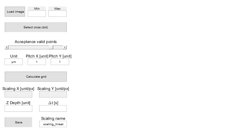
In DefocusTracking, you have a interactive windows to calculated the scaling factors from a picture of a calibration grid of known dimension. In this example we used a calibration grid with a 100 um pitch. Open the windows and try the following steps:

Run command: dtracker_create('scaling')
Load image '.Datasets-WTE2\Grid-100um\B00001.tif'
Push 'select cross'
Select a square around a cross, double click on the rectangle to confirm
Insert the Pitch value (100 and 100)
Insert the unit ('um')
Push 'Calculate grid'
Insert Z Depth: (51-1)*2*1.33
Inser Dt: 10
Insert scaling name: scaling_wte2
Push 'Save'

dtracker_create('scaling')

6 - Run the full processing on all datasets

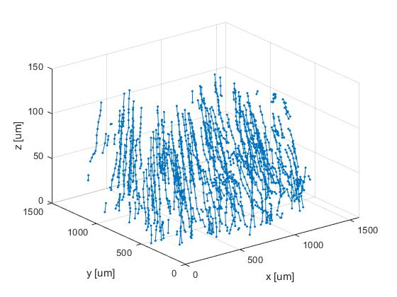
Once you have checked that all your settings are right on few images, you can run the full processing on the entire imageset. In DefocusTracker you can append the tracking and scaling to your model, by creating the field 'tracking' and 'scaling'. Or if you prefer you can do that in separate steps as done so far. You can always apply a new scaling and a new tracking to a dataset.

%  Add the tracking and scaling to the model
model_wte2.tracking = tracking_wte2;
model_wte2.scaling = scaling_wte2;

%  Run the processing on all data frames
dat_exp = dtracker_process(model_wte2,img_exp);

%  Plot the tracks
figure
dtracker_show(dat_exp,'plot_3d_tracks')

Evaluation started ...
1/21 - 7 s - 83 particles - time left: 2 mins, 25.5 secs
2/21 - 7 s - 79 particles - time left: 2 mins, 12.3 secs
3/21 - 7 s - 85 particles - time left: 2 mins, 14.8 secs
4/21 - 7 s - 81 particles - time left: 2 mins, 5.0 secs
5/21 - 8 s - 83 particles - time left: 2 mins, 8.4 secs
6/21 - 8 s - 79 particles - time left: 1 min, 54.3 secs
7/21 - 8 s - 92 particles - time left: 1 min, 54.7 secs
8/21 - 8 s - 89 particles - time left: 1 min, 48.8 secs
9/21 - 9 s - 83 particles - time left: 1 min, 42.4 secs
10/21 - 7 s - 85 particles - time left: 1 min, 21.4 secs
11/21 - 8 s - 87 particles - time left: 1 min, 16.5 secs
12/21 - 7 s - 99 particles - time left: 1 min, 5.5 secs
13/21 - 7 s - 93 particles - time left: 59.9 secs
14/21 - 8 s - 88 particles - time left: 52.9 secs
15/21 - 7 s - 89 particles - time left: 43.1 secs
16/21 - 8 s - 97 particles - time left: 38.1 secs
17/21 - 8 s - 90 particles - time left: 32.8 secs
18/21 - 8 s - 89 particles - time left: 22.9 secs
19/21 - 8 s - 92 particles - time left: 16.7 secs
20/21 - 8 s - 99 particles - time left: 7.6 secs
21/21 - 8 s - 92 particles - time left:  
----------------------------
Evaluation done! Total Time: 2 mins, 42.0 secs
Tracking - nearest neighbor - started...
Tracking done! Total time: 0 min 0 sec

7 - Save the data

Congratulation, you get your first experimental results with DefocusTracer! Do not forget to save all your relevant data! In part 2 of WTE2 you will learn to correct bias and make nicer plots of your data.

myfolder = './/Datasets-WTE2';
save(myfolder,'dat_train','dat_valid','dat_exp','model_wte2')

Bibliography

Interfacial flows in sessile evaporating droplets of mineral water, M. Rossi, A. Marin, and C.J. Kähler, Phys. Rev. E 100, 033103 (2019).

General Defocusing Particle Tracking: Fundamentals and uncertainty assessment, R. Barnkob and M. Rossi, Exp. Fluids 61, 110 (2020).

A fast and robust algorithm for general defocusing particle tracking, M. Rossi and R. Barnkob, Meas. Sci. Technol. 32, 014001 (2020).