WTE1 - Localize 3D particle positions on synthetic data

In this tutorial you will perform your first GDPT analysis and use DefocusTracker to localize the 3D position (X,Y,Z) of particles created with MicroSIG, a synthetic particle image generator. Synthetic particle images are useful to assess the uncertainty of a PTV method since give access to true positions.

You will use all three fundamental data structres of DefocusTracker - imageset, dataset, and model - and all the five basic functions - dtracker_create(), dtracer_show(), dtracker_train(), dtracker_process(), and dtracker_postprocess() -.

Contents

0 - Instruction

1 - Load the imagesets

For this example, you need to create two imagesets. The first imageset contains the training images stored in the folder 'Dataset-WTE1\Calib-noise0'. The second imageset contains the images to be analyzed and are stored in the folder 'Dataset-WTE1\Data-overlapping-noise0-particles1100\'.

clc, clear, close all

%  Create the *imageset* for the training images
myfolder = './/Datasets-WTE1//Calib-noise0//';
img_train = dtracker_create('imageset',myfolder);

% Create the *imageset* for the experimental images
myfolder = './/Datasets-WTE1//Data-overlapping-noise0-particles1100//';
img_test = dtracker_create('imageset',myfolder);

2 - Create a training set

The calibratoin philosophy of DefocusTracker is based on training set of data, following machine learning principle. A training set in DefocusTracker always consists of a pair of imageset and dataset.

For the method used in this tutorial, the training set must consitst of:

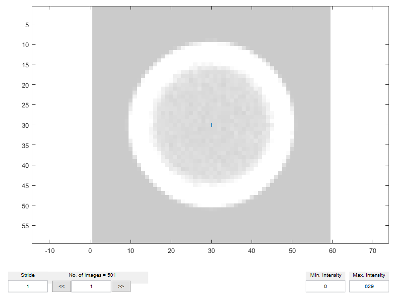
In the current example, in the training imageset we have a sequence of 501 images, but we select a sequence with a stride of 10 frames.

selected_frames = 1:10:501;
N_cal = length(selected_frames);

%  Initialize the *dataset*
dat_train = dtracker_create('dataset',N_cal);

%  Center coordinate of the calibration particle image
dat_train.X(:) = zeros(1,N_cal) + 30;
dat_train.Y(:) = zeros(1,N_cal) + 30;

%  By convention, in DefocusTracker the (unscaled) Z coordinates have values
%  normalized with the total measurement height, thus between 0 and 1.
dat_train.Z(:) = linspace(0,1,N_cal);
dat_train.fr(:) = selected_frames;

%  Check set using dtracker_show(). The blu cross indicate the particle
%  center
dtracker_show(img_train,dat_train)

3 - Create and train the model

Once we have prepared the training set, we can train one model using the dtracker_train() function.

Each method has its own training parameters wich are organized in the following mandatory sub-fields:

In this example we will use the default method of DefocustTracker, method_1. We can specify different methods in the create function: mymodel = dtracker_create('model','mymethod')

%  Create a model using the default method:
model_wte1 = dtracker_create('model');

%  Change the necessary user-editable training parameters
model_wte1.training.imwidth = 51;
model_wte1.training.imheight = 51;

%  Train the model
model_wte1 = dtracker_train(model_wte1,img_train,dat_train);

%  Show the model
dtracker_show(model_wte1)

Training started ...
Training done! Total Time: 0.8 secs

You can look at the calibration images in the bottom left panels. The other panels contain more technical information about the calibration but can also be ignored. For more information we refer to Barnkob & Rossi, Exp Fluids 61, 110 (2020).

4 - Process an imageset with a trained model

In DefocusTracker, an evaluation is performed using the function dtracker_process():

mydataset = dtracker_process(mymodel,myimageset)

dtracker_process() takes as inputs a model and an imageset, and gives as output a dataset.

To evaluate only a subset of the imageset you can use an optional input variable which is a vector with the indices of the frames to be processed (Example in WTE2).

mydataset = dtracker_process(mymodel,myimageset,myframes)

%  Set the processing parameters
model_wte1.processing.cm_guess = .4;
model_wte1.processing.cm_final = .5;

%  Process all images in the "noise0_p500_images" *imageset*
dat_test = dtracker_process(model_wte1, img_test);

%  Display the *dataset* resulting from the processing
figure
dtracker_show(dat_test,'plot_3d')

Evaluation started ...
1/19 - 10 s - 423 particles - time left: 3 mins, 1.8 secs
2/19 - 10 s - 417 particles - time left: 2 mins, 45.0 secs
3/19 - 10 s - 423 particles - time left: 2 mins, 41.4 secs
4/19 - 10 s - 444 particles - time left: 2 mins, 29.6 secs
5/19 - 12 s - 443 particles - time left: 2 mins, 42.3 secs
6/19 - 14 s - 422 particles - time left: 2 mins, 57.8 secs
7/19 - 10 s - 426 particles - time left: 2 mins, 2.3 secs
8/19 - 9 s - 417 particles - time left: 1 min, 40.3 secs
9/19 - 10 s - 430 particles - time left: 1 min, 41.4 secs
10/19 - 10 s - 431 particles - time left: 1 min, 32.5 secs
11/19 - 9 s - 445 particles - time left: 1 min, 15.8 secs
12/19 - 9 s - 418 particles - time left: 1 min, 6.4 secs
13/19 - 10 s - 434 particles - time left: 59.7 secs
14/19 - 9 s - 424 particles - time left: 47.3 secs
15/19 - 10 s - 442 particles - time left: 38.3 secs
16/19 - 11 s - 450 particles - time left: 34.0 secs
17/19 - 11 s - 420 particles - time left: 21.7 secs
18/19 - 11 s - 443 particles - time left: 10.9 secs
19/19 - 10 s - 429 particles - time left:  
----------------------------
Evaluation done! Total Time: 3 mins, 15.6 secs

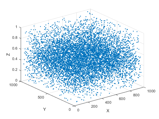
CONGRATULATIONS! You have now successfully performed a GDPT evaluation using DefocusTracker

NOTE: You may notice that the evaluation is not the same everywhere, but there is a small band where less particles are detected. This is due to a particle image shape which is harder to detect in that region. For a deeper discussion on these aspects we refer to Barnkob & Rossi, Exp Fluids 61, 110 (2020).

5 - (Optional) Check the error on true dataset

In this case, since we used synthetic images, we know the true values and we can calculate the error in our measurement. More details on how the error is estimated are given in Barnkob & Rossi, Exp Fluids 61, 110 (2020).

Remember that X, Y, Z are in normalized units:

with M_x magnification in the x-direction, M_y magnification in the y-direction, pixel_size side length of one pixel sensor, and h is the depth of the measurement volume.

NOTE: You can import and export datasets in ASCII file by using the table functions readtable and datatable. In this way however the metadata of the dataset will be lost.

dat_true = readtable('.//Datasets-WTE1//true_coordinates.txt');

[errors, errors_delta] = dtracker_postprocess('compare_true_values',...
   dat_test,dat_true);

disp('          ')
disp('------ Error analysis (result / expected)------')
disp(['Error for X = ',num2str(errors.sigma_X,'%0.3f'),' / 0.440'])
disp(['Error for Y = ',num2str(errors.sigma_Y,'%0.3f'),' / 0.443'])
disp(['Error for Z = ',num2str(errors.sigma_Z,'%0.3f'),' / 0.020'])
disp(['Recall = ',num2str(errors.recall,'%0.3f'),' / 0.330'])

Error evaluation started...
Error evaluation done!
          
------ Error analysis (result / expected)------
Error for X = 0.440 / 0.440
Error for Y = 0.443 / 0.443
Error for Z = 0.020 / 0.020
Recall = 0.330 / 0.330

Bibliography

General Defocusing Particle Tracking: Fundamentals and uncertainty assessment, R. Barnkob and M. Rossi, Exp. Fluids 61, 110 (2020).

A fast and robust algorithm for general defocusing particle tracking, M. Rossi and R. Barnkob, Meas. Sci. Technol. 32, 014001 (2020).

Synthetic image generator for defocusing and astigmatic PIV/PTV, Meas. Sci. Technol. 31, 017003 (2020).

Published with MATLAB® R2020a